A filter of an image is when we layer the centre pixel of a kernel over every pixel in an image. We then multiply each pixel value with its respective kernel value, sum them all up, and divide by the total value of the kernel.
TL;DR, take the average of the sum of all values in the kernel.
A mean blur kernel simplest form of kernel; each value of the kernel is 1, so every pixel used by the kernel is summed and divided linearly.
\[ \begin{bmatrix} 1 & 1 & 1\\ 1 & 1 & 1\\ 1 & 1 & 1 \end{bmatrix} \]
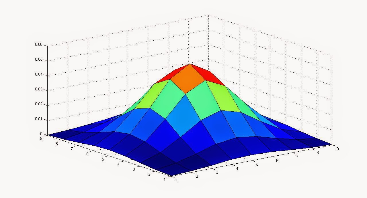
A more complex example of kernel is one with a normal distribution. The gaussian blur is a 2-dimensional normal distribution

It might look something like this:
\[ \begin{bmatrix} 0.25 & 0.5 & 0.25\\ 0.5 & 1 & 0.5\\ 0.25 & 0.5 & 0.25 \end{bmatrix} \]
A gaussian kernel prioritises the pixels in the centre of the kernel
When using kernels in Neural Networks, the values that we apply to the kernels are completely random. This is because each value in the network can be considered a weight.
To provide an image to a network (for example, a multi-layer perceptron), we have to provide every Red, Green, and Blue value of each pixel as an input node. For a 2MP image, that’s 3 \(\times\) 2,000,000 = 6,000,000 inputs, which isn’t realistic for a simple neural network to compute.
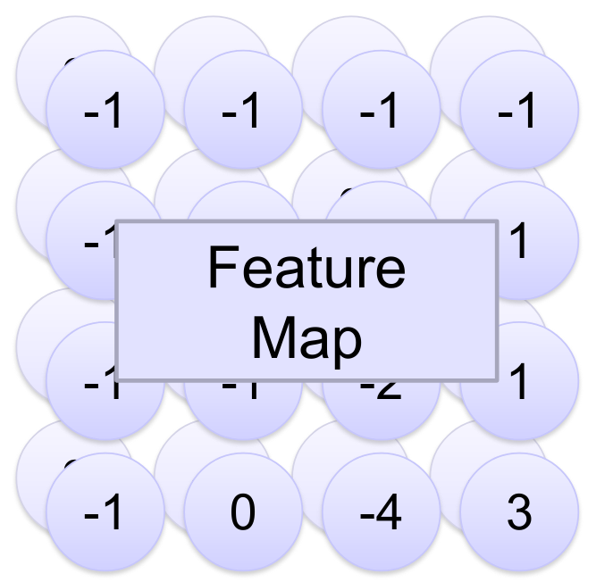
Instead, we pass the image through multiple different kernels, each one returning another image. This is our first feature map, called so because it’s a map of features that the neural network thinks is important. In essence, it’s our first layer of the convolutional network.

We can reduce the resolution between layers of the feature map through a process called Max Pooling by changing the max pool’s dimensions and stride .
We run each layer through another set of convolutions, increasing the number of feature images in the feature map, but reducing each image’s resolution. We do this until each feature map is \(1\times 1\).
These final features can now be represented as nodes, which are fully connected to an output node that returns a single value (or a few values depending on your aims).
We create an \(n \times n\) filter that will be our max pooling filter. Then, we define a stride. Then, we run the filter against the convoluted image once again, but instead of stepping by one each time, we step by the value of our stride.
We store the maximum value of each filter in the corresponding location in the output image.
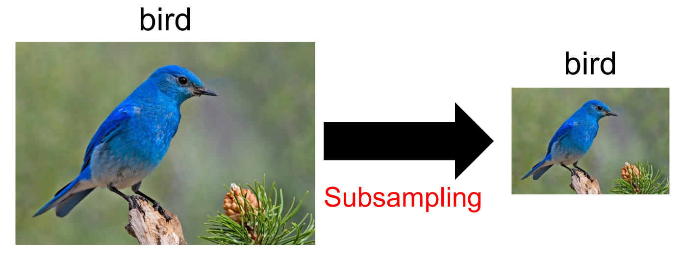
This process is essentially subsampling:

This is the process of adjusting the weights of each kernel’s value based on a prediction on what will reduce the error. This is similar to how a multi-layer perceptron performs back-propagation, using derivations of formulae.