Decision Trees

Decision trees can operate with non-numerical data.

Building a decision tree amounts to deciding the order in which the decisions should be made.

Surprise

Surprise inversely related to probability:

\[ s(x) = \log \Bigg\lparen\frac{1}{p(x)}\Bigg\rparen \]

Writing like this has a few useful benefits:

• If \(p(x) = 0\), \(s(x) =\) undefined, which is okay because it’s not useful to denote surprise for something that can never happen.
• If \(p(x) = 1\), \(s(x) = 0\), showing that there is no surprise that \(x\) will always occur.

Calculating / Estimating Surprise

The surprise of a sequence of events is the sum of the surprise for each individual event:

\[ s(a,a,b) = s(a) + s(a) + s(b) \]

Entropy

The above video explains:

• The entropy of an event is the surprise of that event divided by the number of times it was performed.
• Because calculating the surprise of \(n\) events multiplies by \(n\), and calculating the entropy of such surprise divides by \(n\), then entropy cancels out and becomes the following formula:

\[ \text{Entropy} = \sum_{i = 0}^n p(x_i) \log_2 \Bigg\lparen\frac{1}{p(x)}\Bigg\rparen \]

• Since \(\log(\frac{a}{b}) = \log(a) - \log(b)\), this is more commonly written as:

\[ \text{Entropy} = -\sum_{i = 0}^n p(x_i) \log_2 \Big(p(x_i)\Big) \]

Heads & Tails Example

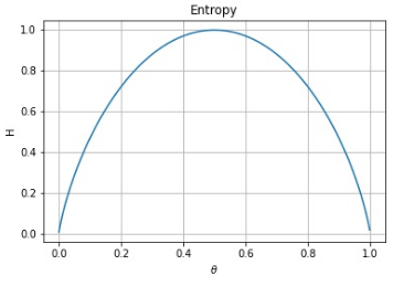
Say we have a random binary variable \(x \in \{\text{Heads},\text{Tails}\}\), and \(\theta\) is the probability \(p(x = \text{Heads})\). The entropy \(H\) can be plotted as follows:

You can see that entropy reduces as the probability approaches 0 and 1. That is to say, if we are more certain that a particular outcome will happen, entropy decreases.

Information Gain

When building a decision tree, we want the next decision to have a large impact on the entropy towards 0. The Information gain tells us how important a given attribute \(x_i\) is. It is used to decide the order in which to place an attribute.

Information Gain \(G(S,F)\) is defined as follows, where \(S\) is the set of elements and \(F\) is the set of features:

\[ G(S,F) = \text{Entropy}(S) - \sum_{f \in F} \frac{|S_f|}{|S|} \text{Entropy}(S_f) \]

Information Gain should be as high as possible over a decision tree.

Gini Impurity of a Set

Algorithms

ID3

Computes the information gain for every possible feature in the set \(F\) and chooses the one that produces the highest value, outputting a complete decision tree.

1. Calculate the Information Gain of each feature.
2. Considering that all rows don’t belong to the same class, split the dataset S into subsets using the feature for which the Information Gain is maximum.
3. Make a decision tree node using the feature with the maximum Information gain.
4. If all rows belong to the same class, make the current node as a leaf node with the class as its label.
5. Repeat for the remaining features until we run out of all features, or the decision tree has all leaf nodes.

CART

Glossary

• Information: The amount of surprise in an outcome with a given probability \(p_i\). \(I_i = -\log_2(p_i)\)
• Entropy: The amount of expected surprise in an outcome with a given probability. \(H = E[I] = \sum_i -p_i \log_2(p_i)\)